Category: Uncategorized
Apache Lucene is a Java toolkit that provides a rich set of search capabilities like keyword search, query suggesters, relevancy, and faceting. It also has a spatial module for searching and sorting with geometric data using either a flat-plane model or a spherical model. For the most part, the capabilities therein are leveraged to varying degrees by Apache Solr and ElasticSearch–the two leading search servers based on Lucene.
Advanced spatial
The most basic and essential spatial capability is the ability to index points specified using latitude and longitude, and then be able to search for them based on a maximum distance from a given query point—often a users location, or the center of a maps viewport. Most information-retrieval systems (e.g. databases) support this.
Most relational databases, such as PostGIS, are mature and have advanced spatial support. I loosely define advanced spatial as the ability to both index polygons and query for them by another polygon. Outside of relational databases, very few information-retrieval systems have advanced spatial support. Some notable members of the advanced spatial club are Lucene, Solr, Elasticsearch, MongoDB and Apache CouchDB. In this article we’ll be reviewing advanced spatial in Lucene.
How it works…
This article describes how polygon indexing & search works in some conceptual detail with pointers to specific classes. If you want to know literally how to use these features in Lucene, then first know you should be familiar with Lucene. Find a basic tutorial on that if you arent familiar with it. Then you should read the documentation for the Lucene-spatial API, and review the SpatialExample.java source which shows some basic usage. Next, read the API Javadocs referenced here within the article for relevant classes. If instead you want to know how to use it from Solr and ElasticSearch, this isnt the right article, not to mention that the new accurate indexing addition isnt yet hooked into those search servers yet, as of this writing.
Grid indexing with PrefixTrees
From Lucene 4 through 4.6, the only way to index polygons is to use Lucene-spatial’s PrefixTreeStrategy which is an abstract implementation of SpatialStrategy — the base abstraction for how to index and search spatially. It has two subclasses, TermQueryPrefixTreeStrategy and RecursivePrefixTreeStrategy (RPT for short) — I always recommend the latter. The indexing scheme is fundamentally based on a model in which the world is divided into grid squares (AKA cells), and is done so recursively to get almost any amount of accuracy required. Each cell, is indexed in Lucene with a byte string that has the parent cell’s byte string as a prefix — hence the name PrefixTree.
The PrefixTreeStrategy uses a SpatialPrefixTree abstraction that decides how to divide the world into grid-squares and what the byte encoding looks like to represent each grid square. There are two implementations:
- geohash: This is strictly for latitude & longitude based coordinates. Each cell is divided into 32 smaller cells in an 8×4 or 4×8 alternating grid.
- quad: Works with any configurable range of numbers. Each cell is divided into 4 smaller cells in a straight-forward 2×2 grid.
We’ll be using a geohash based PrefixTree for the examples in this article. For further information about geohashes, to include a convenient table of geohash length to accuracy, go to Wikipedia.
Indexing points
Lets now see what the indexed bytes look like in the geohash SpatialPrefixTree grid for indexing a point. We’ll use Boston Massachusetts: latitude 42.358, longitude -71.059. If we go to level 5, then we have a grid cell that covers the entire area ± 2.4 kilometers from its center (about 19 square kilometers in this case):
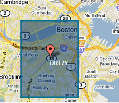
This will index as the following 5 “terms” in the underlying Lucene index:
D, DR, DRT, DRT2, DRT2YTerms are the atomic byte sequences that Lucene indexes on a per-field basis, and they map to lists of matching documents (i.e. records); in this case, a document representing Boston.
If we attempt to index any other hypothetical point that also falls in the cell’s boundary it will also be indexed using the same terms, effectively coalescing them into the same for search purposes. Note that the original numeric literals are returned in search results since they are internally stored separately.
To get more search accuracy we need to take the PrefixTree to more levels. This easily scales: there aren’t that many terms to index per point. If you want accuracy of about a meter then level 11 will do it, translating to 11 indexed terms. The search algorithms to efficiently search grid squares indexed in this way are interesting but it’s not the focus of this article.
Indexing other shapes
The following screen-captures depict the leaf cells indexed for a polygon of Massachusetts to a grid level of 6 (±0.61km from center):
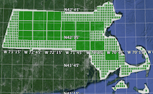
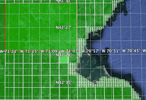
The biggest cells here are at level 4, and the smallest are at 6. A leaf cell is a cell that is indexed at no smaller resolution, either because it doesn’t cross the shape’s edge, or it does but the accuracy is capped (configurable). There are 5,208 leaf cells here. Furthermore, when the shape is indexed, all the parent (non-leaf) cells get indexed too which adds another 339 cells that go all the way up to coarsest cell “D”. The current indexing scheme calls for leaf cells to be indexed both with and without a leaf marker — an additional special ‘+’ byte. The grand total number of terms to index is 10,755 terms. That’s a lot! Needless to say, we won’t list them here.
Note: the extra indexed term per leaf will get removed in the future, once the search algorithms are adapted for this change. See LUCENE-4942.
Theoretically, to get more accuracy we “just” need to go to lower grid levels, just as we do for points. But unless the shape is small relative to the desired accuracy, it doesn’t scale; it’s simply infeasible with this indexing approach to represent a region covering more than a few square kilometers to meter level accuracy. Each additional PrefixTree level multiplies the number of indexed terms compared to the previous level. The Massachusetts example went to level 6 and produced 5208 leaf cells, but if it had just gone to level 5 then there would have been only 463 leaf cells. With each additional level, there will be on average 32 / 2 = 16 times as many (for geohash) cells of the previous level. For a quad-tree it’s 4 / 2 = 2 times as many, but it also takes more than one added level of a quad tree to achieve the same desired accuracy, so it’s effectively the same no matter how many leaves are in the tree.
Summary: unlike a point shape, which has a linear relationship between accuracy and the number of terms, polygon shapes are exponential to the power of the numbers of levels. This clearly doesn’t scale for high-accuracy requirements.
Serialized shapes
Lucene 4.7 introduced a new Lucene-spatial SpatialStrategy called SerializedDVStrategy (SDV for short). It serializes each documents shape vector geometry itself into a part of the Lucene Index called DocValues. At query time, candidate results are verified as true or false matches, by retrieving the geometry by doc-id on-demand, deserializing, and comparing to the query shape.
As of this writing, there aren’t any adapters for ElasticSearch or Solr yet. The Solr feature request is tracked as SOLR-5728, and is probably going to arrive in Solr 4.9. The adapters will likely maintain in-memory caches of deserialized shapes to speed up execution.
Using both strategies
It’s critical to understand that SerializedDVStrategy is not a PrefixTree index; if used alone, SerializedDVStrategy will brute-force and deserialize compare all documents, O(N) complexity, and have terrible spatial performance.
In order to minimize the number of documents that SerializedDVStrategy has to see, you should put a faster SpatialStrategy like RecursivePrefixTreeStrategy in front of it. And you can now safely dial-down the configurable accuracy of RPT to return more false-positives since SDV will filter them out. This is done with the distErrPct option, which is roughly the fraction of a shape’s approximate radius, and it defaults to 0.025 (2.5%). Given the Massachusetts polygon, RPT arrived at level 6. If distErrPct is changed to 0.1 (10%), my recommendation when used with SDV, the algorithm chose level 5 for Massachusetts, which had about 10% as many cells as level 6.
Performance and accuracy — the holy grail
What I’m most excited about is the prospect of further enhancing the PrefixTree technique such that it is able to differentiate matching documents between those that are a guaranteed matches versus those that need to be verified against the serialized geometry. Consider the following shape, a circle, acting as the query shape:
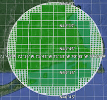
If any grid cell that isn’t on the edge matches a document, then the PrefixTree guarantees it’s a match; there’s no point in checking such documents against SerializedDVStrategy (SDV). This insight should lead to a tremendous performance benefit since a small fraction of matching documents, often zero, will need to be checked against SDV. Performance and accuracy! This feature is being tracked with LUCENE-5579.
One final note about accuracy — it is only as accurate as the underlying geometry. If you’ve got a polygon representation of an area with only 20 vertices, and another with 1000 for the same area, then more vertices are likely to be a more precise reflection of the border of the underlying area. Secondly, you might want to work in a projected 2D coordinate system instead of latitude & longitude. Lucene-spatial / Spatial4j / JTS doesn’t help in this regard, it’s up to your application to convert the coordinates with something such as Proj4j. The main shortcoming of this approach is that a point-radius (circle) query is going to be in 2D even if you might have wanted a geodesic (surface of a sphere) implementation that normally happens when you use latitudes & longitudes. But if you are projecting then the distorted difference between the two is generally fairly limited if the radius isn’t large and if the area isn’t near the poles.
Acknowledgements
Thanks to the Climate Corporation for supporting my recent improvements for accurate spatial queries!